
There are few things in financial analysis quite as amusing as watching someone draw a straight line across a stock chart and then proceed to explain the future of the global economy with the confidence of an astronomer predicting an eclipse.
Apparently, all you need to understand the financial markets is a ruler, a chart, and a willingness to ignore everything that doesn’t fit your theory.
Draw a line connecting two peaks. Extend it into the future. Congratulations! You’ve discovered resistance.
Connect a couple of troughs. Extend that line, too. Congratulations again! You’ve discovered support.
Find three points that happen to fall somewhere near a straight line, and you’ve discovered a trend.
And if the market subsequently moves in the direction of your line, you’re a genius. If it doesn’t, you probably just need to redraw it.
Welcome to the astrology of financial analysis.
The Magic of Connecting the Dots
The fundamental problem with drawing lines on financial charts is that markets don’t move in straight lines. They move through a constantly changing interaction of buyers, sellers, liquidity, leverage, interest rates, earnings expectations, sentiment, economic conditions, and an almost endless number of other variables.
Yet somehow, we’re supposed to believe that connecting a few historical price points reveals an underlying geometric structure that predicts where the market is going.
Consider what happens when you look at a chart after the fact.
You can select two peaks and draw a descending resistance line. You can select two troughs and draw an ascending support line. You can choose different peaks and troughs and produce an entirely different set of lines.
All of them will look perfectly reasonable.
That’s the problem.
The line doesn’t reveal the pattern. The analyst creates the pattern by choosing which points to connect.
Even if you manage to fudge enough peaks and troughs into something resembling a perfectly linear trend, what have you actually demonstrated? Only that, among thousands of possible ways to connect historical data points, you found a handful that happen to line up.
That’s not predictive analysis. That’s retrospective geometry.
And the more freedom you give yourself to choose the starting points, ending points, timeframes, and chart scales, the easier it becomes to find something that looks meaningful.
Example 1: The Same Chart, Trendlines Going in Every Direction
One of the most absurd aspects of trendline analysis is that the direction of the trend often depends entirely on how far back you choose to look.
Zoom in on a stock chart, and you can find an upward trend. Zoom out a little, and suddenly you’re looking at a downward trend. Expand the timeframe further, and you might discover an entirely different long-term upward channel.
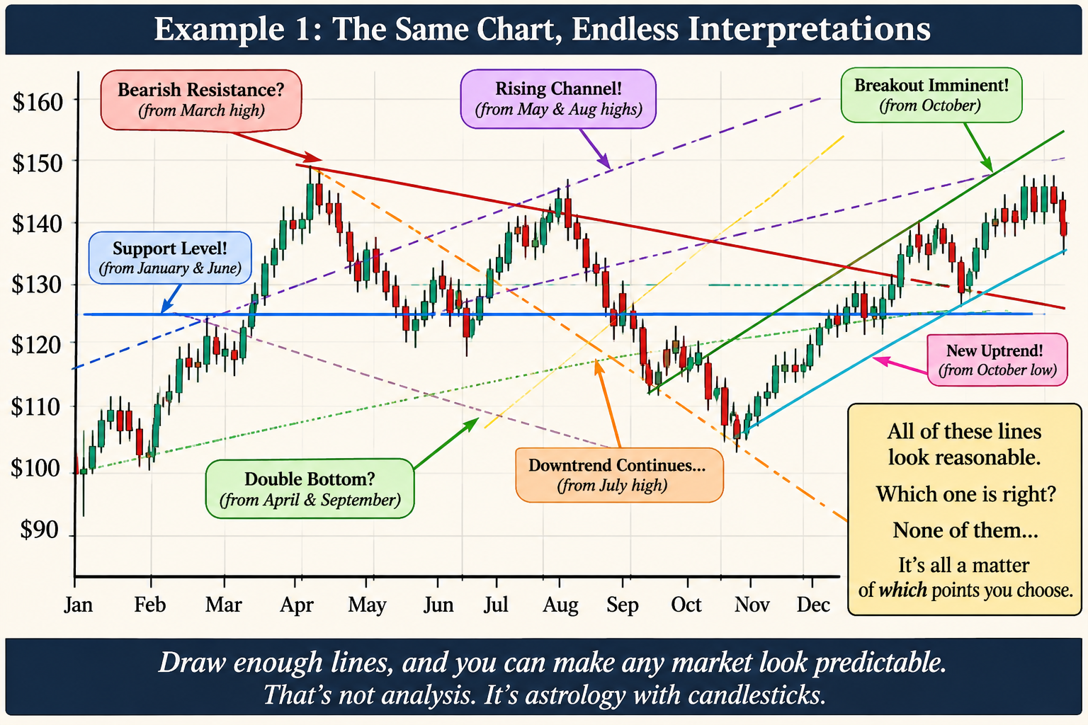
The same thing happens when selecting which peaks and troughs to connect. Start at the January low and connect it to a June low, and you’ve got ascending support. Start at the April high and connect it to the August high, and you’ve got descending resistance. Choose a couple of different points, and you can manufacture another bullish channel, bearish channel, breakout pattern, or support level.
Before long, your chart looks like a plate of spaghetti.
And every line has a perfectly reasonable explanation.
- Bullish trend: Connect the lows from January and June.
- Bearish trend: Connect the highs from April and August.
- New breakout: Use the September low as your starting point.
- Long-term resistance: Extend a line from an earlier market peak.
- Support level: Draw a horizontal line through a handful of previous lows.
Which one is correct? Depending on the timeframe and the points selected, all of them can appear equally convincing.
This is the fundamental problem with hand-drawn trendlines: there is no objective rule determining which points matter, which timeframe is relevant, or how much deviation from a line is acceptable. The analyst gets to choose all of those things after seeing the data.
You can always zoom in until you find a bullish trend, or zoom out until you find a bearish one. You can redraw the lines whenever the market moves, and if one interpretation stops working, simply find another.
But none of this tells you where the market is actually going.
A trendline is just a geometric relationship between selected historical prices. It doesn’t establish that those prices share a meaningful relationship, that other market participants recognize the same line, or that future prices have any reason to follow it.
If changing the zoom level or selecting different historical points can produce a completely different prediction, what exactly is the predictive value of the line?
Draw enough lines across enough timeframes, and you can make virtually any market look bullish, bearish, or ready to break out.
That’s not discovering a trend. It’s manufacturing one. causation. It could just as easily be coincidence, ordinary volatility, or the result of other market forces.
Example 2: The Endless Search for a Perfect Trendline
Here’s another problem: the further back you look, the easier it becomes to find a trendline.
Take a chart with several years of price history. You can draw a line through the lows of one particular market cycle, another through the lows of a different cycle, and perhaps a third through a few intermediate points.
Depending on your selection, the market might appear to be:
- In a long-term bullish trend.
- In a bearish correction.
- Breaking out of a consolidation.
- Approaching a major resistance level.
- Retesting a previous support level.
The same historical data can tell five different stories.
And there’s no shortage of technical analysts willing to explain why their particular line is the correct one.
This is a classic example of hindsight bias and data mining: searching historical data until you find a relationship that looks meaningful, then treating that relationship as though it had predictive power all along.
The problem is well documented in academic research. In their 2000 paper, Foundations of Technical Analysis, Andrew Lo, Harry Mamaysky, and Jiang Wang identified the subjective nature of chart interpretation as one of the major obstacles to evaluating technical analysis. They noted that geometric patterns in historical charts are often in the eye of the beholder.
A 2023 study by Guglielmo Caporale and Alex Plastun, Seven Pitfalls of Technical Analysis, likewise identified subjectivity, data snooping, statistically insignificant results, and unrealistic simplifications among its major shortcomings.
Example 3: If You Can Draw It Afterward, It Doesn’t Mean You Could Predict It Beforehand
Let’s say the S&P 500 experiences a major correction.
After the market bottoms, an analyst draws a line connecting the previous lows and announces that the market has established a new ascending support channel.
The market rallies. The line appears validated.
A few months later, the market experiences another correction and breaks below the line.
Now the analyst has several options:
- Declare the trend broken.
- Redraw the line using a different set of lows.
- Switch to a longer timeframe.
- Explain that the market temporarily violated support but has not invalidated the broader trend.
Notice what’s happening.
The original prediction was based on a line that could be adjusted whenever reality failed to cooperate.
If a theory can be continually modified to accommodate every possible outcome, it isn’t much of a predictive theory.
A useful analytical method should establish its rules before the outcome is known. It should be measurable, repeatable, and capable of being proven wrong.
If two analysts examining the same data cannot agree on where the trendline belongs, the methodology has a serious problem.
Financial Markets Are Not Linear Systems
Perhaps the biggest misconception behind trendline analysis is the assumption that financial markets behave in a relatively orderly, linear fashion.
They don’t.
Market behavior is influenced by multiple interacting variables, often in ways that are nonlinear, conditional, and constantly changing.
Consider just a few examples:
Volatility clustering: Large price movements tend to be followed by periods of elevated volatility, while quiet periods often persist. Market volatility doesn’t simply increase or decrease along a straight line.
Momentum and mean reversion: Markets can exhibit momentum over certain periods and mean-reverting behavior over others. A price movement that initially reinforces a trend can eventually produce exhaustion and reversal.
Liquidity and leverage: A relatively small change in liquidity can have a disproportionate effect on prices when leveraged positions begin unwinding. A market can move from relatively stable to disorderly very quickly.
Regime changes: Markets behave differently during periods of monetary expansion, tightening, recession, financial crisis, and speculative exuberance. A relationship that appears to work under one set of conditions may become completely unreliable under another.
Research published in The European Journal of Finance in 2021, titled Nonlinearity Everywhere: Implications for Empirical Finance, Technical Analysis and Value at Risk, examines how nonlinear relationships in financial markets can make simple linear models misleading.
This is important because a straight line drawn across historical prices assumes a degree of continuity that simply cannot be taken for granted.
Markets are dynamic systems, not geometry exercises.
What About Technical Indicators?
This isn’t to say that all technical indicators are useless. There is a substantial difference between drawing arbitrary lines on a chart and calculating indicators from defined mathematical relationships.
Consider a few examples:
Relative Strength Index (RSI)
RSI doesn’t simply connect a series of price peaks. It compares average gains and losses over a specified period and transforms their ratio into a bounded oscillator between zero and 100.
It can help identify changes in momentum and potential overbought or oversold conditions. Its value comes from a defined calculation, not from an analyst deciding which two points look important.
Average True Range (ATR)
ATR measures volatility using true range, which accounts for the relationship between the current high and low and the previous closing price. It incorporates gaps and is typically smoothed over time.
It provides a quantitative measure of how much an asset is moving, rather than assuming volatility can be represented by a straight line.
Moving Average Convergence Divergence (MACD)
MACD compares two exponential moving averages and uses their difference to examine changes in momentum. Its signal line and histogram provide additional information about the relationship between those averages.
Bollinger Bands
Bollinger Bands combine a moving average with standard deviations to create dynamically adjusting boundaries around price. As volatility changes, the bands expand and contract.
These indicators aren’t magic, either. They can produce false signals, lag behind price movements, and fail under changing market conditions. Some are mathematically linear components, while others involve nonlinear transformations. But they are at least defined, reproducible calculations that can be tested.
And that’s the important distinction.
A legitimate indicator has a formula. You can calculate it, compare it across different assets and timeframes, backtest it, and evaluate whether it provides useful information.
A hand-drawn trendline has an analyst.
The Power of Combining Indicators: Fibonacci, Bollinger Bands, and MACD
If we’re going to take technical analysis seriously, we should at least focus on tools that measure something meaningful.
Some of the more interesting approaches involve combining indicators rather than relying on a single measurement. In particular, Fibonacci retracement levels, Bollinger Bands, and MACD can provide complementary perspectives on price behavior.
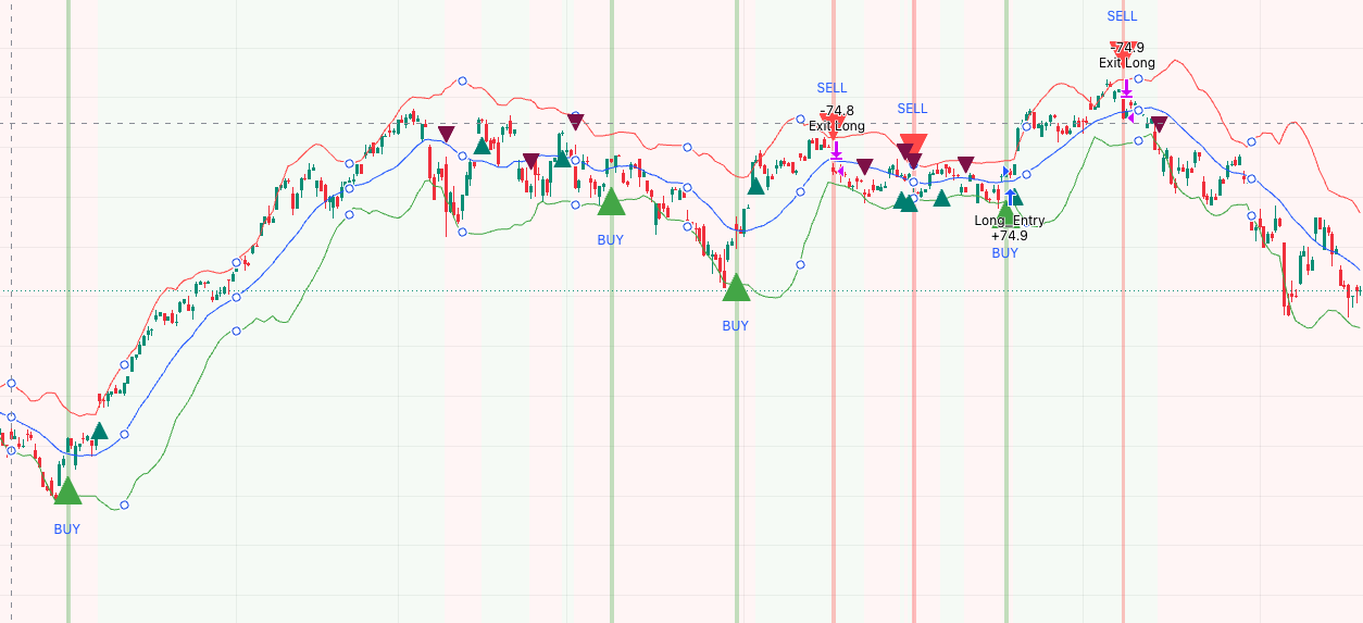
Fibonacci retracements identify mathematical price levels based on ratios derived from the Fibonacci sequence, most commonly 38.2%, 50%, and 61.8%. These levels can help identify areas where a correction might encounter buying or selling pressure. Unlike arbitrary trendlines, Fibonacci levels are calculated according to a defined methodology. Of course, the selection of the original swing high and low still involves judgment, and the levels themselves aren’t magical.
Bollinger Bands measure price relative to a moving average and its standard deviation. They expand when volatility increases and contract when volatility decreases. This makes them useful for understanding changing volatility regimes, identifying periods of compression, and examining whether price movements are unusually extended relative to recent conditions.
MACD (Moving Average Convergence Divergence) examines the relationship between two exponential moving averages. It provides insight into momentum, including whether momentum is strengthening, weakening, or changing direction.
Individually, each indicator has limitations. Together, however, they can provide a more comprehensive picture.
For example, imagine a market declining toward a Fibonacci retracement level while simultaneously approaching the lower Bollinger Band. If MACD is also showing declining downside momentum or a bullish crossover, the combination presents a potentially interesting setup.
Three different measurements are telling a somewhat consistent story:
- Fibonacci identifies a potential price area of interest.
- Bollinger Bands provide context about volatility and relative price extension.
- MACD provides information about momentum and its direction.
This doesn’t guarantee a reversal. It simply provides multiple pieces of measurable evidence that can be evaluated together.
Another interesting combination is Bollinger Bands with MACD. A Bollinger Band squeeze can identify a period of contracting volatility, while MACD can help assess the direction and strength of momentum as the market begins to move. The combination can be particularly useful for examining potential breakouts, although neither indicator can reliably predict when a breakout will occur or whether it will succeed.
The important distinction is that these indicators are based on explicit mathematical calculations. Their behavior can be measured, their signals can be tested, and their limitations can be evaluated.
Even Fibonacci levels, which involve some subjective selection of swing points, offer a reproducible calculation once those points are established.
That’s a considerably better starting point than drawing a line through three convenient peaks and declaring you’ve discovered the future.
The real opportunity in technical analysis isn’t finding increasingly creative ways to draw lines. It’s combining independent measurements of price, volatility, and momentum to develop a more complete understanding of market behavior.
The Problem Isn’t Just the Lines. It’s the Confidence.
There’s nothing inherently wrong with visualizing historical prices. Charts are useful. They help us understand what has happened, compare different periods, and identify changes in market behavior.
The problem arises when someone mistakes a visual coincidence for a predictive relationship.
If a market happens to touch a particular price level three times, that doesn’t mean the fourth touch will produce a reversal.
If a series of peaks happens to align, that doesn’t mean the next peak will follow the same trajectory.
If you can draw a channel around historical price movements, that doesn’t mean the market is obligated to remain inside it.
And if you need to adjust your line every time the market moves, perhaps the line wasn’t telling you very much to begin with.
There may be legitimate statistical relationships behind certain price patterns. Some forms of technical analysis have demonstrated incremental predictive information under particular conditions. But that is an argument for rigorous measurement and testing, not for treating every geometric coincidence as a revelation.
A trading strategy should be evaluated using explicit rules, realistic transaction costs, risk management, and out-of-sample testing. It should demonstrate that it works on data it wasn’t designed around.
Otherwise, you’re just drawing pictures of the past.
Conclusion: Put Away the Ruler
Financial markets are complicated. Their behavior reflects the interaction of countless variables, many of which change over time. Understanding them requires mathematics, statistics, probability, and an appreciation for the limitations of predictive models.
It doesn’t require a ruler.
You can draw as many lines as you want. You can connect every peak, every trough, every intermediate high, and every convenient low. Eventually, you’ll find something that looks like a pattern.
But finding a pattern in historical data isn’t the same as discovering a law of nature.
And predicting where the market will go based on a line you drew through where it has already been is a little like predicting tomorrow’s weather by connecting yesterday’s clouds.
It’s not analysis. It’s astrology with candlesticks.
The market doesn’t care about your trendlines.